scenarioMonteCarloAttRW

Overview

Demonstrates how to run basic Monte-Carlo (MC) RW-based attitude simulations. This script duplicates the scenario in scenarioAttitudeFeedbackRW where a 6-DOF spacecraft is orbiting the Earth. Here some simulation parameters are dispersed randomly using a multi threaded Monte-Carlo setup. Reaction Wheel (RW) state effector are added to the rigid spacecraftPlus() hub, and what flight algorithm module is used to control these RWs. The scenario is run in a single configuration: by not using the Jitter model and by using the RW Voltage IO. Given this scenario we can add dispersions to the variables in between each MC run.

The script is found in the folder src/examples and executed by using:

python3 scenarioMonteCarloAttRW.py

For more information on the Attitude Feedback Simulation with RW, please see the documentation on the scenarioAttitudeFeedbackRW file.

Setup Changes for Monte-Carlo Runs

In order to set up the multi-threaded MC simulation, the user must first instantiate the Controller class. The function that is being simulated is the set in this class (in this case, it’s defined in the same file as the MC scenario). The user can then set other variables such as the number of runs, the dispersion seeds, and number of cores.

The next important step to setting up the MC runs is to disperse the necessary variables. The dispersions that are set are listed in the following table:

Input	Description of Element	Distribution
Inertial attitude	Using Modified Rodrigues Parameters	Uniform for all 3 rotations between [0, 2 pi]
Inertial rotation rate	Using omega vector	Normal dispersions for each of the rotation components, each of mean 0 and standard deviation 0.25 deg/s
Mass of the hub	Total Mass of the spacecraft	Uniform around +/-5% of expected values. Bounds are [712.5, 787.5]
Center of Mass Offset	Position vector offset on the actual center of mass, and its theoretical position	Normally around a mean [0, 0, 1], with standard deviations of [0.05/3, 0.05/3, 0.1/3]
Inertia Tensor	3x3 inertia tensor. Dispersed by 3 rotations	Normally about mean value of diag(900, 800, 600). Each of the 3 rotations are normally distributed with angles of mean 0 and standard deviation 0.1 deg.
RW axes	The rotation axis for each of the 3 wheels	Normally around a respective means [1,0,0], [0,1,0], and [0,0,1] with respective standard deviations [0.01/3, 0.005/3, 0.005/3], [0.005/3, 0.01/3, 0.005/3], and [0.005/3, 0.005/3, 0.01/3].
RW speeds	The rotation speed for each of the 3 wheels	Uniform around +/-5% of expected values. Bounds are [95, 105], [190, 210], and [285, 315]
Voltage to Torque Gain	The gain between the commanded torque and the actual voltage	Uniform around +/-5% of expected values. Bounds are [0.019, 0.021]

Next a retention policy is used to log the desired data. The simulation can now be run. It returns the failed jobs, which should not occur. When the MC have been executed, the data can be accessed and tested in different ways. This is explained in the example python code comments.

Illustration of Simulation Results

saveFigures = False, case = 1, show_plots = True, useDatashader = False

Datashader and Monte Carlo

To install the datashader capability, see the Installing Optional Packages. Using datashader and holoviews together can rasterize and visualize large amounts of data very quickly. We have provided a generalized datashader interface for Monte Carlo runs in the utilities folder called datashaderGraphingInterface. After installing datashader and importing it in your monte carlo, you can incorporate into a Monte Carlo very easily. First you need a method that you can easily call to configure the datashader library. In this Monte Carlo, this method is called configureDatashader(). It is referenced at the top of the run(...) function. An additional argument has been added to run(...) called usedatashader. This is set either in the pytest script or in the __main__ function of the Monte Carlo.

The script first checks to see if the datashader library is installed on the computer. Next, you have to set the callback function to call a method within datashader Library instead of using the callback in the Monte Carlo. Then, set the Monte Carlo to show plots using datashader instead of matplotlib. Lastly, populate the configureDatashader() with the graphs and data that the library will graph. This is done by creating a list of Graph objects, and passing them to datashaderLibrary.

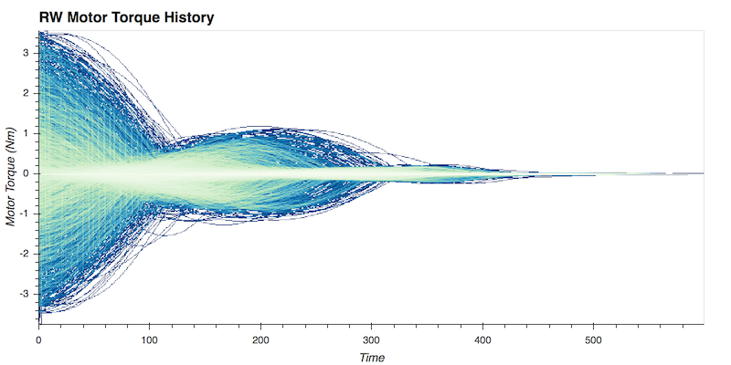
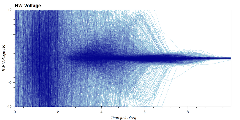
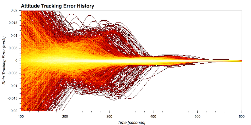
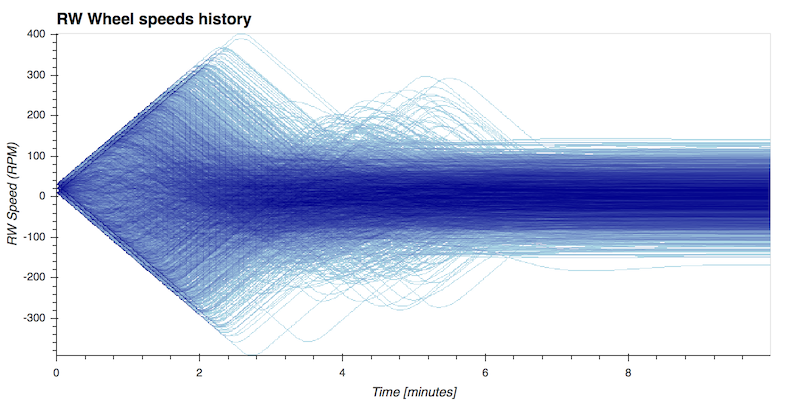
There are inherently two different ways to save the graphs with the datashaderLibrary using either Holoviews or Datashader. The default is using holoviews, which rasterizes the data via datashader, and saves all of the graphs into an html file. From there, graphs can be saved as png files by opening the html file in a browser, and clicking the save button. Graphs that are generated by holoviews (which also uses bokeh, and datashader) and will look like this:

The second method of visualization only uses dat``ashader, and therefore is not wrapped around a graphing library. This will result in higher quality images; however, they do not have axis values, labels, etc. All you generate is solely an image. Here are some of the datashaded images that are from the same data as the holoview graphs above:

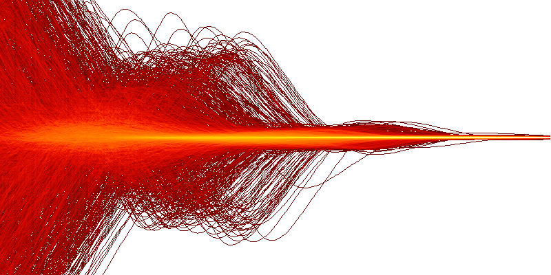
Attitude Error Datashaded

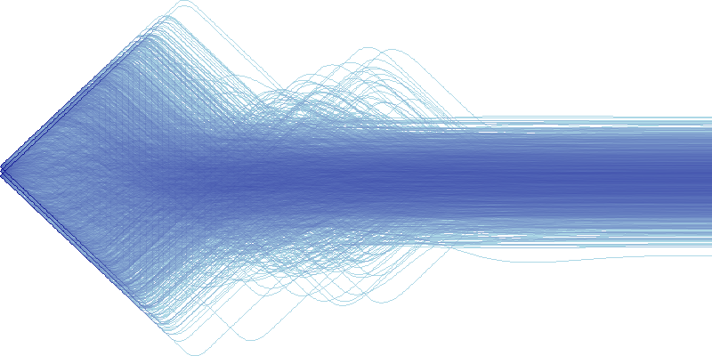
Reaction Wheel Speeds

Here are some examples of the Attitude Error in different color with a set x and y range to zoom in on the data.

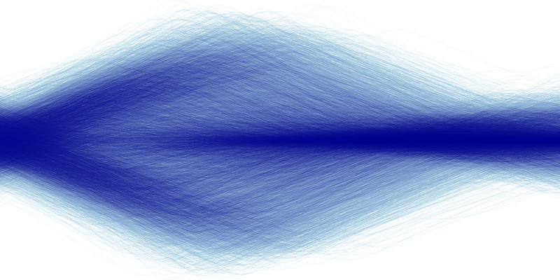
Default color shading

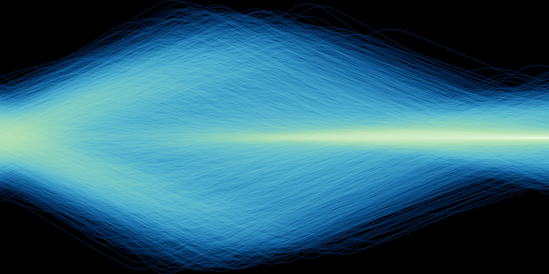
GNU Color shading

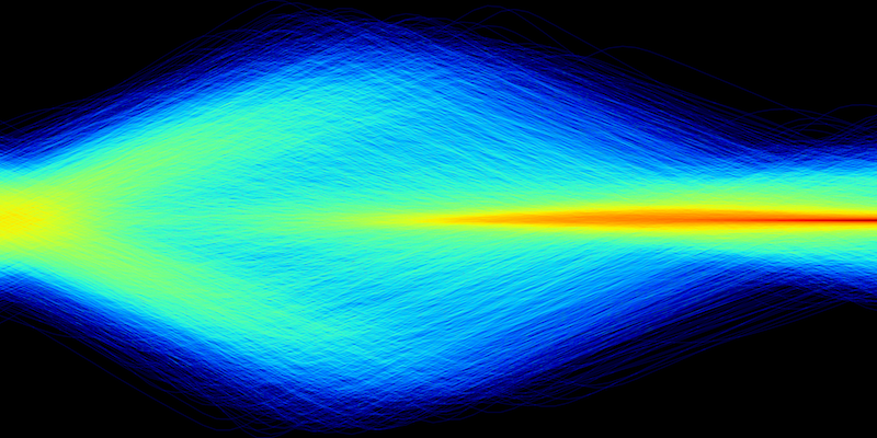
Jet color Shading

These are the same plots output by the scenarioMonteCarloAttRW scenario. Please refer to this document for me details on the plots.

scenarioMonteCarloAttRW.run(saveFigures, case, show_plots, useDatashader)

The scenarios can be run with the followings setups parameters:

Parameters

• saveFigures (bool) – flag if the scenario figures should be saved for html documentation

• case (int) – Case 1 is normal MC, case 2 is initial condition run

• show_plots (bool) – Determines if the script should display plots

• useDatashader (bool) – Flag to do the plotting using python datashader package